---

overreact is a library and a command-line tool for building and analyzing homogeneous microkinetic models from first-principles calculations:

In [1]: from overreact import api  # the api

In [2]: api.get_k("S -> E‡ -> S",  # your model
   ...:           {"S": "data/ethane/B97-3c/staggered.out",  # your data
   ...:            "E‡": "data/ethane/B97-3c/eclipsed.out"})
Out[2]: array([8.16880917e+10])  # your results

The user specifies a set of elementary reactions that are believed to be relevant for the overall chemical phenomena. overreact offers a hopefully complete but simple environment for hypothesis testing in first-principles chemical kinetics.

🤔 What is microkinetic modeling?

Microkinetic modeling is a technique used to predict the outcome of complex chemical reactions. It can be used to investigate the catalytic transformations of molecules. overreact makes it easy to create and analyze microkinetic models built from computational chemistry data.

🧐 What do you mean by first-principles calculations?

We use the term first-principles calculations to refer to calculations performed using quantum chemical modern methods such as Wavefunction and Density Functional theories. For instance, the three-line example code above calculates the rate of methyl rotation in ethane (at B97-3c). (Rather surprisingly, the error found is less than 2% when compared to available experimental results.)

overreact uses precise thermochemical partition funtions, tunneling corrections and data is parsed directly from computational chemistry output files thanks to cclib (see the list of its supported programs).

Installation

overreact is a Python package, so you can easily install it with pip:

$ pip install "overreact[cli,fast]"

See the installation guide for more details.

🚀 Where to go from here? Take a look at the short introduction. Or see below for more guidance.

Citing overreact

If you use overreact in your research, please cite:

Schneider, F. S. S.; Caramori, G. F. Overreact, an in Silico Lab: Automative Quantum Chemical Microkinetic Simulations for Complex Chemical Reactions. Journal of Computational Chemistry 2022, 44 (3), 209–217. doi:10.1002/jcc.26861.

Here's the reference in BibTeX format:

@article{overreact_paper2022,
  title         = {Overreact, an in silico lab: Automative quantum chemical microkinetic simulations for complex chemical reactions},
  author        = {Schneider, Felipe S. S. and Caramori, Giovanni F.},
  year          = {2022},
  month         = {Apr},
  journal       = {Journal of Computational Chemistry},
  publisher     = {Wiley},
  volume        = {44},
  number        = {3},
  pages         = {209–217},
  doi           = {10.1002/jcc.26861},
  issn          = {1096-987x},
  url           = {http://dx.doi.org/10.1002/jcc.26861},
}
@software{overreact_software2021,
  title         = {geem-lab/overreact: v1.1.0 \vert{} Zenodo},
  author        = {Felipe S. S. Schneider and Let\'{\i}cia M. P. Madureira and  Giovanni F. Caramori},
  year          = {2023},
  month         = {Jan},
  publisher     = {Zenodo},
  doi           = {10.5281/zenodo.7504800},
  url           = {https://doi.org/10.5281/zenodo.7504800},
  version       = {v1.1.0},
  howpublished  = {\url{https://github.com/geem-lab/overreact}},
}

License

overreact is open-source, released under the permissive MIT license. See the LICENSE agreement.

Funding

This project was developed at the GEEM lab (Federal University of Santa Catarina, Brazil), and was partially funded by the Brazilian National Council for Scientific and Technological Development (CNPq), grant number 140485/2017-1.

Where to go next

💡 If you want to...

...install the software ➡️ read the installation instructions.

...learn the basics ➡️ take a look at the tutorial.

...use it as a command-line tool to model a reaction ➡️ read the command-line reference.

...learn about the command-line input format ➡️ read the input format reference.

...use it as a library ➡️ take a look at the available example Jupyter notebooks.

...read about how it works ➡️ read our simple description.

Installing overreact

The recommended way of installing the package is from the command line using pip:

$ pip install overreact

✏️ You may need to call pip3 instead of pip.

The above command will install a minimal set of features. If you plan to use the command-line interface, you have to specify the cli extra feature:

$ pip install overreact[cli]

💡 If you would like to use automatic differentiation (through Google's JAX library) instead of the default numerical differentiation, you have to specify the fast extra feature as well:
$ pip install overreact[cli,fast]

Dependencies

overreact depends on:

cclib (parser for computational chemistry logfiles).
SciPy (numerical integration, optimization, unit conversion and others).

✏️ Don't worry, these dependencies are automatically installed when you install overreact using pip as indicated above.

As stated above, extra functionality is provided such as a command-line interface. If you would like to install the full set of supported features, you can specify the following extra flags:

$ pip install overreact[cli,fast]

The line above installs Rich (used in the command-line interface) and JAX (speeds up calculations) as well.

⚠️ An extra solvents flag is available that adds some solvent properties by means of the thermo library. It is not fully integrated into the package yet: it is meant to provide, in the future, dynamic viscosities for solvents in the context of the Collins-Kimball theory for diffusion-limited reactions (Journal of Colloid Science, 1949, 4, 425–437; Industrial & Engineering Chemistry, 1949, 41, 2551–2553). Stay tuned and, if you are interested, let's discuss it!

Troubleshooting

Can't install overreact: `pip: command not found` or similar

You may need to install pip on your system.

💡 The pip developers have provided an excellent installation guide for you.

Can't run overreact: `overreact: command not found` or similar

If you get this error, two things could be happening:

1️⃣ You haven't properly installed the package.

To fix this first problem, take a look at a previous section. If you're running a Unix, you can check if the package is installed by running pip list | grep overreact:

$ pip list | grep overreact
overreact 1.1.0

Alternatively, you can try to import the package directly from Python:

$ python
Python 3.9.7 (default, Sep 10 2021, 14:59:43)
[GCC 11.2.0] on linux
Type "help", "copyright", "credits" or "license" for more information.
>>> import overreact
>>> overreact.__version__
'1.1.0'

2️⃣ You are missing the `overreact` command in your `PATH`.

To fix this, you have to add the pip executable directory (i.e. the place where pip puts executables during installation) to your PATH. For example, if you installed overreact using pip install overreact as indicated above, the overreact executable will be inside ~/.local/bin.

This can be solved by adding the following line to your ~/.bashrc file (or ~/.zshrc if you use zsh):

export PATH="$HOME/.local/bin:$PATH"

💡 Read more about PATH on the Unix & Linux Stack Exchange.

Quickstart

This is a step-by-step guide on using overreact as a command-line tool. It will teach you all the basics of overreact through a guided use-case.

\[\require{mhchem}\]

A simple Curtin-Hammett system

We're going to explore a system that is simple enough to be a tutorial, but also interesting enough to show off most of the capabilities of overreact. The reaction is a classical SN$_2$ reaction on a substituted cyclohexane:

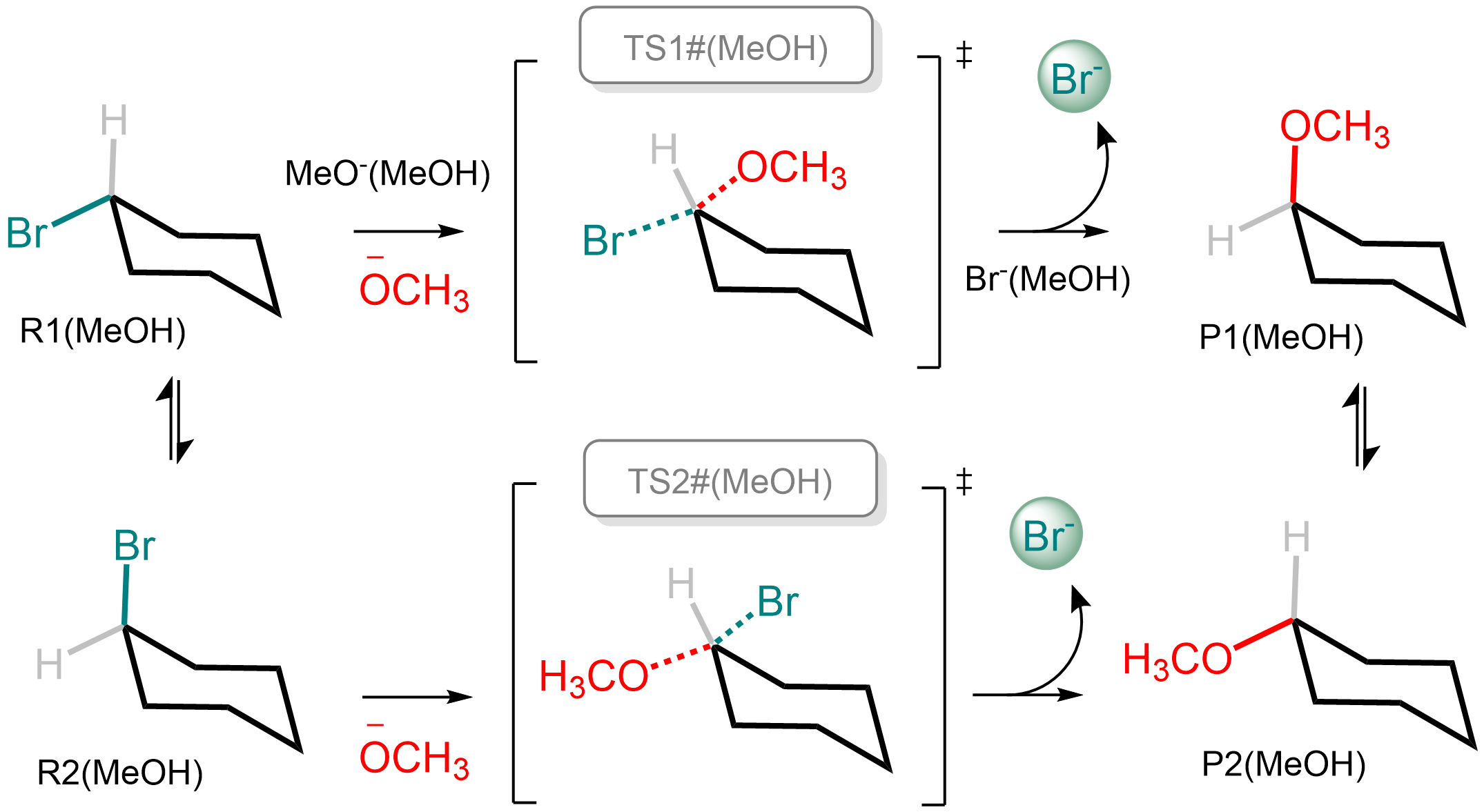
The labels above refer to the file names and the labels in the input file below. The steps above were calculated using GFN2-xTB by calling the Semiempirical Extended Tight-Binding Program Package (XTB) from within ORCA 4.2.1. Methanol was used as (implicit) solvent.

💡 You can download a zip file of this tutorial to run everything yourself.

Step 1: Create the input file

Inside the zip file, you'll find an input file called methoxylation.k. It contains the following:

// methoxylation.k

// This is a comment.

$scheme
 // Here we define our reactions.
 R1(MeOH) <=> R2(MeOH)
 P1(MeOH) <=> P2(MeOH)
 R1(MeOH) + MeO-(MeOH) -> TS1#(MeOH) -> P1(MeOH) + Br-(MeOH)
 R2(MeOH) + MeO-(MeOH) -> TS2#(MeOH) -> P2(MeOH) + Br-(MeOH)
$end

$compounds
 // The path to the logfiles go here.
 R1(MeOH):   R1@MeOH/opt+numfreq.out
 R2(MeOH):   R2@MeOH/opt+numfreq.out
 P1(MeOH):   P1@MeOH/opt+numfreq.out
 P2(MeOH):   P2@MeOH/opt+numfreq.out
 MeO-(MeOH): MeO-@MeOH/opt+numfreq.out
 TS1#(MeOH): TS1@MeOH/b/optts+numfreq.out
 Br-(MeOH):  Br-@MeOH/singlepoint.out
 TS2#(MeOH): TS2@MeOH/b/optts+numfreq.out
$end

It describes the reactions and the compounds in the system (take a look at a more detailed description of the input format here). The reactions are almost an exact translation of the diagram above (observe the labels in the figure are the same as in the input file).

✏️ Solvation is indicated by the parentheses at the end of compound names. As such, overreact adds corrections for solvation standard states to compounds such as name(solv), where solv is any identifier you want to use. It is good practice to use an identifier that clearly identifies the chemical environment such as name(MeOH).

After performing the calculations, obtaining the logfiles, and writing the input file, it's time to run overreact.

Step 2: Run overreact (or a tour over a typical output)

A first run of overreact would look like this:

$ overreact methoxylation.k

This will produce quite an amount of output, so let's walk through it one step at a time.

2.1: The header

The current version v1.1.0 produces a header similar to the following one:

╔═══════════════════════════════════════════════════════════════════════════════════════════════════════╗
║                                            overreact 1.1.0                                            ║
╚═══════════════════════════════════════════════════════════════════════════════════════════════════════╝

📈 Create and analyze chemical microkinetic models built from computational chemistry data.

Licensed under the terms of the MIT License. If you publish work using this software, please cite
doi:10.5281/zenodo.7504800:

┌───────────────────────────────────────────────────────────────────────────────────────────────────────┐
│                                                                                                       │
│ @misc{overreact2021,                                                                                  │
│   howpublished = {\url{https://github.com/geem-lab/overreact}},                                       │
│   year = {2021},                                                                                      │
│   author = {Schneider, F. S. S. and Caramori, G. F.},                                                 │
│   title = {                                                                                           │
│     \textbf{geem-lab/overreact}: a tool for creating and analyzing                                    │
│     microkinetic models built from computational chemistry data, v1.1.0                               │
│   },                                                                                                  │
│   doi = {10.5281/zenodo.7504800},                                                                     │
│   url = {https://zenodo.org/record/7504800},                                                          │
│   publisher = {Zenodo},                                                                               │
│   copyright = {Open Access}                                                                           │
│ }                                                                                                     │
└───────────────────────────────────────────────────────────────────────────────────────────────────────┘

Read the user guide at https://geem-lab.github.io/overreact-guide/ for more information and usage
examples. Other useful resources:

 • Questions and Discussions
 • Bug Tracker
 • GitHub Repository
 • Python Package Index

─────────────────────────────────────────────────────────────────────────────────────────────────────────
Inputs:

 • Path           = methoxylation.k
 • Concentrations = []
 • Verbose level  = 0
 • Compile?       = False
 • Plot?          = none
 • QRRHO?         = both
 • Temperature    = 298.15 K
 • Pressure       = 101325.0 Pa
 • Integrator     = Radau
 • Max. Time      = 86400
 • Rel. Tol.      = 1e-05
 • Abs. Tol.      = 1e-11
 • Bias           = 0.0 kcal/mol
 • Tunneling      = eckart

The important for us at the moment is the Inputs section. It contains all the information that overreact needs to run the calculations, so that you can check if it's doing what you want.

Then, after some logging, the program prints information on the parsed reactions and compounds.

2.2: The reactions and compounds

For our example, the reactions are:

╭─────────────────────────────────────────────────────────────────╮
│                        (read) reactions                         │
│                                                                 │
│   R1(MeOH) <=> R2(MeOH)                                         │
│   P1(MeOH) <=> P2(MeOH)                                         │
│   R1(MeOH) + MeO-(MeOH) -> TS1#(MeOH) -> P1(MeOH) + Br-(MeOH)   │
│   R2(MeOH) + MeO-(MeOH) -> TS2#(MeOH) -> P2(MeOH) + Br-(MeOH)   │
│                                                                 │
╰─────────────────────────────────────────────────────────────────╯
                                (parsed) reactions

  no   reactant(s)             via‡         product(s)             half equilib.?
 ─────────────────────────────────────────────────────────────────────────────────
   0   R1(MeOH)                             R2(MeOH)                    Yes
   1   R2(MeOH)                             R1(MeOH)                    Yes
   2   P1(MeOH)                             P2(MeOH)                    Yes
   3   P2(MeOH)                             P1(MeOH)                    Yes
   4   R1(MeOH) + MeO-(MeOH)   TS1#(MeOH)   P1(MeOH) + Br-(MeOH)         No
   5   R2(MeOH) + MeO-(MeOH)   TS2#(MeOH)   P2(MeOH) + Br-(MeOH)         No

                     logfiles

  no   compound     path
 ────────────────────────────────────────────────
   0   R1(MeOH)     R1@MeOH/opt+numfreq.out
   1   R2(MeOH)     R2@MeOH/opt+numfreq.out
   2   P1(MeOH)     P1@MeOH/opt+numfreq.out
   3   P2(MeOH)     P2@MeOH/opt+numfreq.out
   4   MeO-(MeOH)   MeO-@MeOH/opt+numfreq.out
   5   TS1#(MeOH)   TS1@MeOH/b/optts+numfreq.out
   6   Br-(MeOH)    Br-@MeOH/singlepoint.out
   7   TS2#(MeOH)   TS2@MeOH/b/optts+numfreq.out

Here we have an opportunity to see the reactions disassembled and the species classified into reactants, products, and transition states. We also classify reactions as being part of an equilibrium reaction or not.

The next data involves the compounds.

2.3: The species

                                          compounds

  no   compound       elec. energy      spin mult.       smallest vibfreqs       point group
                         〈Eₕ〉                              〈cm⁻¹〉
 ────────────────────────────────────────────────────────────────────────────────────────────
   0   R1(MeOH)      -22.576340550900       1         +121.5,  +207.0,  +228.3       Cs
   1   R2(MeOH)      -22.575218880620       1         +111.9,  +174.2,  +238.2       Cs
   2   P1(MeOH)      -26.215281987160       1          +64.1,  +121.7,  +167.1       C1
   3   P2(MeOH)      -26.216556401840       1          +73.0,  +119.6,  +190.9       C1
   4   MeO-(MeOH)     -7.985271579600       1        +1133.7, +1177.9, +1179.5       C3v
   5   TS1#(MeOH)    -30.552250438240       1         -404.8,   +22.4,   +93.7       C1
   6   Br-(MeOH)      -4.435371316770       1                                         K
   7   TS2#(MeOH)    -30.558417149310       1         -451.8,   +55.7,   +86.2       C1

                             estimated thermochemistry (compounds)

  no   compound      mass         Gᶜᵒʳʳ            Uᶜᵒʳʳ            Hᶜᵒʳʳ              S
                    〈amu〉    〈kcal/mol〉     〈kcal/mol〉     〈kcal/mol〉    〈cal/mol·K〉
 ──────────────────────────────────────────────────────────────────────────────────────────────
   0   R1(MeOH)     163.06             80.57           103.35           103.94         78.38
   1   R2(MeOH)     163.06             80.63           103.21           103.80         77.73
   2   P1(MeOH)     114.19            105.68           129.35           129.95         81.39
   3   P2(MeOH)     114.19            105.63           129.38           129.98         81.64
   4   MeO-(MeOH)    31.03              9.96            23.18            23.77         46.33
   5   TS1#(MeOH)   194.09             99.20           127.78           128.37         97.85
   6   Br-(MeOH)     79.90             -8.27             0.89             1.48         32.70
   7   TS2#(MeOH)   194.09             99.77           127.83           128.42         96.11

Here we have the information about the compounds. overreact uses the electronic energy, geometry, atomic masses,vibrational frequencies, charge and spin multiplicity to obtain all it needs to run the calculations. In particular, the point groups are obtained from the geometries and atomic masses. We see that the $\ce{MeO-}$ ion gets classified as $C_{3v}$ and both reactants are $C_s$. Then the next table shows the estimated thermochemistry for the compounds.

Then comes the data about the reactions.

2.4: The reactions

The next two tables show the reaction thermochemistry.

                                                   estimated (reaction°) thermochemistry

  no   reaction                                        Δmass°        ΔG°            ΔE°            ΔU°            ΔH°             ΔS°
                                                       〈amu〉   〈kcal/mol〉   〈kcal/mol〉   〈kcal/mol〉   〈kcal/mol〉   〈cal/mol·K〉
 ──────────────────────────────────────────────────────────────────────────────────────────────────────────────────────────────────────────
   0   R1(MeOH) -> R2(MeOH)                              0.00           0.76           0.70           0.57           0.57           -0.66
   1   R2(MeOH) -> R1(MeOH)                              0.00          -0.76          -0.70          -0.57          -0.57            0.66
   2   P1(MeOH) -> P2(MeOH)                              0.00          -0.85          -0.80          -0.77          -0.77            0.25
   3   P2(MeOH) -> P1(MeOH)                              0.00           0.85           0.80           0.77           0.77           -0.25
   4   R1(MeOH) + MeO-(MeOH) -> P1(MeOH) + Br-(MeOH)    -0.00         -48.99         -55.87         -52.16         -52.16          -10.62
   5   R2(MeOH) + MeO-(MeOH) -> P2(MeOH) + Br-(MeOH)    -0.00         -50.60         -57.38         -53.50         -53.50           -9.71

                                                  estimated (activation‡) thermochemistry

  no   reaction                                        Δmass‡        ΔG‡            ΔE‡            ΔU‡            ΔH‡             ΔS‡
                                                       〈amu〉   〈kcal/mol〉   〈kcal/mol〉   〈kcal/mol〉   〈kcal/mol〉   〈cal/mol·K〉
 ──────────────────────────────────────────────────────────────────────────────────────────────────────────────────────────────────────────
   0   R1(MeOH) -> R2(MeOH)
   1   R2(MeOH) -> R1(MeOH)
   2   P1(MeOH) -> P2(MeOH)
   3   P2(MeOH) -> P1(MeOH)
   4   R1(MeOH) + MeO-(MeOH) -> P1(MeOH) + Br-(MeOH)     0.00          14.55           5.87           7.13           6.54          -26.86
   5   R2(MeOH) + MeO-(MeOH) -> P2(MeOH) + Br-(MeOH)     0.00          10.48           1.30           2.74           2.15          -27.94

The first table shows reaction free energies and its components. The second table shows the activation energies and its components. Equilibria appear as empty lines in the second table.

✏️ Observe that we show the 'mass variation' for each reaction in a dedicated column: it should be full of zeroes. It is a sanity check to make sure that the mass balance is satisfied, which is very useful for catching common mistakes.

Last, we have the kinetic data.

2.5: The kinetic data

                                                     estimated reaction rate constants

  no   reaction                                        half equilib.?         k                     k                      k           κ
                                                                        〈M⁻ⁿ⁺¹·s⁻¹〉   〈(cm³/particle)ⁿ⁻¹·s⁻¹〉   〈atm⁻ⁿ⁺¹·s⁻¹〉
 ──────────────────────────────────────────────────────────────────────────────────────────────────────────────────────────────────────────
   0   R1(MeOH) -> R2(MeOH)                                 Yes               1                     1                      1
   1   R2(MeOH) -> R1(MeOH)                                 Yes             3.63                  3.63                   3.63
   2   P1(MeOH) -> P2(MeOH)                                 Yes             4.16                  4.16                   4.16
   3   P2(MeOH) -> P1(MeOH)                                 Yes               1                     1                      1
   4   R1(MeOH) + MeO-(MeOH) -> P1(MeOH) + Br-(MeOH)         No              159                2.64e-19                  6.5         1.18
   5   R2(MeOH) + MeO-(MeOH) -> P2(MeOH) + Br-(MeOH)         No           1.56e+05              2.59e-16               6.38e+03       1.21

Only in the table above, all Gibbs free energies were biased by 0.0 J/mol.
For half-equilibria, only ratios make sense.

The last table shows the reaction rate constants in three different units. We also have tunneling coefficients for convenience, but they are already included in the kinetic data.

⚠️ The reaction rate constants for equilibrium reactions are not "genuine" rate constants: they are calculated such that the equilibrium constant is satisfied. This is used during the microkinetic simulations. Only their ratios are meaningful.

Section 3: Microkinetic simulations

In order to perform a microkinetic simulation, all we have to do is add an initial condition to the command line:

$ overreact methoxylation.k "R1(MeOH):0.4" "MeO-(MeOH):0.6"

Initial conditions are given as a list of species and their concentrations separated by a colon.

✏️ The names are the same as in the input file and the concentrations are all in molar units.

A new section at the end of the output then appears:

     initial and final concentrations
                  〈M〉

  no   compound     t = 0 s   t = 0.05 s
 ────────────────────────────────────────
   0   R1(MeOH)       0.400        0.000
   1   R2(MeOH)       0.000        0.000
   2   P1(MeOH)       0.000        0.077
   3   P2(MeOH)       0.000        0.323
   4   MeO-(MeOH)     0.600        0.200
   5   TS1#(MeOH)     0.000        0.000
   6   Br-(MeOH)      0.000        0.400
   7   TS2#(MeOH)     0.000        0.000

Simulation data was saved to methoxylation.csv

Here we see a sketch of the initial and final concentrations of the species and the approximate time when the reactions reach completion. A CSV file is created with the simulation data automatically as well, with concentrations as function of time. You can either analyze the data yourself or ask overreact to do a simple plot of the data for you.

3.1: Plot of "active" species

The active species are the ones that actually change their concentration during the simulation. You can ask overreact to plot them for you with the following command:

$ overreact methoxylation.k "R1(MeOH):0.4" "MeO-(MeOH):0.6" --plot=active

💡 You can also request a plot of all species with the --plot=all option, or of a specific species with something like --plot="P1(MeOH)".

The plot is shown immediately in a new window.

Active species

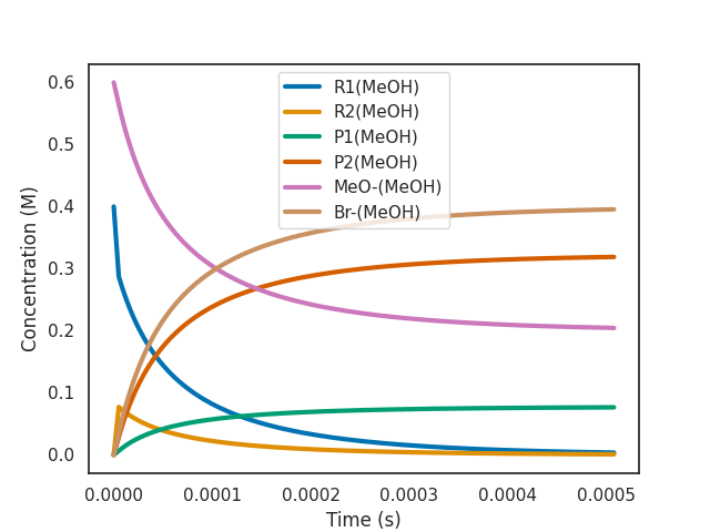
As we can see, the most abundant reactant at the beginning of the simulation is the R1(MeOH). This leads to product P1(MeOH) being formed most of the time. But P1(MeOH) rapidly interconverts to P2(MeOH) and then to R2(MeOH) and back

✏️ The customizations you can do in the command line are necessarily limited and serve mainly to help you explore the data. You can have full control over the plot, simulation parameters, and other factors by using the overreact API directly. Also, take a look at some of the example notebooks.

3.1.1: The effect of a bias

overreact allows one to apply a bias to the Gibbs free energy of all species. This provides a way of counterbalancing systematic errors often found in computed Gibbs free energies, but is also useful for exploring the sensitivity of the generated profiles with respect to unknown error contributions.

In order to insert a bias, you can use the --bias option:

$ overreact methoxylation.k "R1(MeOH):0.4" "MeO-(MeOH):0.6" --plot=active --bias=-4.5

⚠️ Internally, overreact always uses joules/mol, but the bias is always given in kcal/mol for convenience.

Active species with bias

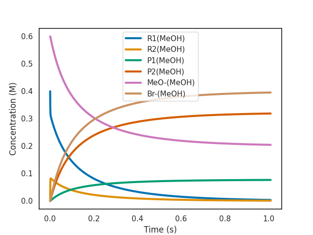
As we can see from the plot above, a bias of -4.5 kcal/mol makes the reaction 2000x slower (as expected from $\exp(4.5 \text{ kcal$\cdot$mol$^{-1}$} / R T) \approx 1989$ at room temperature for a bimolecular reaction).

Jupyter notebooks

We provide a collection of Jupyter notebooks that you can use to explore the application programming interface (API) and learn more about using overreact as a Python library. The example notebooks are available in the notebooks folder at GitHub. The following notebooks are available:

💬 If you have any questions about the notebooks, don't hesitate to open a discussion about it in the overreact GitHub repository.

How it works

overreact takes computational chemistry outputs as data sources and uses them to calculate thermodynamic and kinetic properties as shown in the following diagram below.

graph TD
    class A,B,C,D,E,F,G,H,data,cond,hypo,init,pred normal

    data[/Data sources/] -.-> A[Free energy data <br> for all species];
    cond[/Conditions/] -.-> E;
    hypo[/Reaction hypotheses/] -.->|parser| G[Reaction network];
    init[/Initial concentrations/] -.-> D;
    cond -.-> A;

    subgraph inputs
        data
        cond
        hypo
        init
    end

    G --> F[Reaction rate laws] --> C[Reaction rate equations];
    A --> B[Free energy data for reactions];
    B --> E[Reaction rate constants] --> C --> D((ODE solver));
    G --> B;

    subgraph overreact
        A
        B
        C
        D
        E
        F
        G
    end

    D -.->|scipy| pred;
    pred -->|outputs| H[Kinetic predictions];


    pred[\Concentrations for all species as a function of time\]

WARNING: This above diagram greatly simplifies things. It is not a complete description of the system and in no way substitutes the full read of the upcoming paper.

Using overreact as a command-line tool

✏️ This an overview of the command-line tool. If you're new to overreact, you probably want to go over the tutorial first.

Most commonly, you'll use the command-line tool to manage, explore and analyze your microkinetic simulations. The following is a brief overview of options available in the command-line tool. You can access the full help page by running overreact --help. The output as of version 1.1.0 will be something similar to the following:

$ overreact --help
usage: overreact [-h] [--version] [-v] [-c] [--plot PLOT] [-b BIAS]
                 [--tunneling {eckart,wigner,none}]
                 [--no-qrrho {both,enthalpy,entropy,none}] [-T TEMPERATURE]
                 [-p PRESSURE] [--method {Radau,BDF,LSODA}]
                 [--max-time MAX_TIME] [--rtol RTOL] [--atol ATOL]
                 path [concentrations ...]

📈 Create and analyze chemical microkinetic models built from computational
chemistry data. Read the user guide at https://geem-lab.github.io/overreact-guide/
for more information and usage examples. Licensed under the terms of
the MIT License. If you publish work using this software, please cite
https://doi.org/10.5281/zenodo.7504800.

positional arguments:
  path                  path to a source (`.k`) or compiled (`.jk`) model input
                        file (if a source input file is given, but there is a
                        compiled file available, the compiled file will be
                        used; use --compile|-c to force recompilation of the
                        source input file instead)
  concentrations        (optional) initial compound concentrations (in moles
                        per liter) in the form 'name:quantity' (if present, a
                        microkinetic simulation will be performed; more than
                        one entry can be given) (default: None)

optional arguments:
  -h, --help            show this help message and exit
  --version             show program's version number and exit
  -v, --verbose         increase output verbosity (can be given many times,
                        each time the amount of logged data is increased)
                        (default: 0)
  -c, --compile         force recompile a source (`.k`) into a compiled (`.jk`)
                        model input file (default: False)
  --plot PLOT           plot the concentrations as a function of time from the
                        performed microkinetics simulation: can be either
                        'none', 'all', 'active' species only (i.e., the ones
                        that actually change concentration during the
                        simulation) or a single compound name (e.g. 'NH3(w)')
                        (default: none)
  -b BIAS, --bias BIAS  an energy value (in kilocalories per mole) to be added
                        to each individual compound in order to mitigate
                        eventual systematic errors (default: 0.0)
  --tunneling {eckart,wigner,none}
                        specify the tunneling method employed (use
                        --tunneling=none for no tunneling correction)
                        (default: eckart)
  --no-qrrho {both,enthalpy,entropy,none}
                        disable the quasi-rigid rotor harmonic oscillator
                        (QRRHO) approximations to both enthalpies and
                        entropies (see [doi:10.1021/jp509921r] and
                        [doi:10.1002/chem.201200497]) (default: both)
  -T TEMPERATURE, --temperature TEMPERATURE
                        set working temperature (in kelvins) to be used in
                        thermochemistry and microkinetics (default: 298.15)
  -p PRESSURE, --pressure PRESSURE
                        set working pressure (in pascals) to be used in
                        thermochemistry (default: 101325.0)
  --method {Radau,BDF,LSODA}
                        integrator used in solving the ODE system of the
                        microkinetic simulation (default: Radau)
  --max-time MAX_TIME   maximum microkinetic simulation time (in s) allowed
                        (default: 86400)
  --rtol RTOL           relative local error of the ODE system integrator
                        (default: 1e-05)
  --atol ATOL           absolute local error of the ODE system integrator
                        (default: 1e-11)

The following is a brief description of the most commonly used options:

The path to the model input file

The command-line tool requires the path to either a model source file (.k) or a compiled one (.jk), from which it will read the given logfiles and calculate all the thermodynamic and kinetic quantities of interest.

💡 Click here to learn all about the syntax of the model source file format.

⚠️ overreact compiles your model (i.e., generates .jk files from the .k ones you've written) and tries to use the compiled ones whenever they are available. If you want to force recompilation of the source file (e.g., your .k has changed), you can use the --compile or -c option (see below).

Initial concentrations

All the remaining positional arguments are considered initial concentrations of compounds in the model. They are given in the form name:quantity, where name is the name of a compound (defined in the model source file) and quantity is the number of moles of that compound per liter of the working fluid (i.e., concentrations are given in moles per liter).

If at least one initial concentration is given, a microkinetic simulation will be performed, and the concentrations of the model species at the end of the simulation will be printed to the standard output.

⚠️ Kinetic profiles (e.g., plots of concentrations as a function of time) won't be produced by default. You should use the --plot option in order to produce kinetic profiles (see below).

Produce kinetic profiles 📈

The --plot flag can be used to produce kinetic profiles (e.g., plots of concentrations as a function of time during the microkinetic simulation).

You can either plot all the species (--plot=all) or only the active ones (i.e., the ones that actually change concentration during the simulation, up to a reasonable threshold, --plot=active) or a single compound of interest (--plot="NH3(w)").

Energetics, kinetics and bias correction

The flags --temperature (or -T) and --pressure can be used to set the working temperature and pressure, respectively, to be used in all thermodynamic and kinetic calculations. Units are in kelvins and pascals, respectively, and the default values are 298.15 K and 101.325 kPa.

The --qrrho flag can be used to enable or disable the quasi-rigid rotor harmonic oscillator (QRRHO) approximations for entropies (Theory. Chem. Eur. J., 2012, 18: 9955-9964)) and enthalpies (J. Phys. Chem. C 2015, 119, 4, 1840–1850)). The default value is both, which means that both entropies and enthalpies will be corrected, but you can also choose to only enable the correction for entropies (--qrrho=entropy) or only for enthalpies (--qrrho=enthalpy), or to disable the correction altogether (--qrrho=none).

Quantum tunneling approximations can be selected or disabled with the --tunneling flag. The default value is eckart (for the Eckart model), and other valid options are --tunneling=wigner (Wigner model) and --tunneling=none (no tunneling correction).

A bias energy (in kilocalories per mole) can be added to the model to mitigate eventual systematic errors by using --bias (or -b). This will add a constant energy value to each individual compound in the model. This is zero by default.

⚠️ You should probably have a good reason to add a bias energy correction to your model.

Force recompilation of the source file

The --compile (or, equivalently, -c) option forces the recompilation of the source file (.k) into a compiled (.jk) model input file. This is useful if you want to make sure you're using the latest version of the source file.

🤔 Why doesn't overreact recompile my model automatically?

This is a design decision. The reason is that overreact is designed to work with very large models, and they can be slow interpret (imagine a model with a lot of reactions and a lot of species; overreact would have to read every logfile every time you run it, which can be quite slow).

Tuning the integrator

Some options are available to tune the integrator used in solving the microkinetic ODE system:

The --method flag can be used to specify the integrator to be used (possible values are Radau, BDF and LSODA). The default is Radau.
The --rtol and --atol flags can be used to override the default relative and absolute local errors of the ODE system integrator (the default values are $10^{-5}$ and $10^{-11}$, respectively, which can be given in scientific notation as --rtol=1e-5 and --atol=1e-11).
The --max-time flag can be used to specify the maximum microkinetic simulation time (in seconds) allowed (the default is 86400 seconds, or one day)

Take a look at the documentation of the scipy.integrate.solve_ivp function for low-level details on the integrator options.

Command-line input format specification

overreact is both a library and a command-line application. In this subsection, we briefly describe the minimal input specification for the command-line application for doing first-principles microkinetic simulations. Don't worry, the input is very simple, yet flexible.

Basically, overreact parses complex reaction schemes with the help of a domain-specific language (DSL) designed to be as flexible and intuitive as possible to any chemist. For instance, as a purely illustrative example, the following Curtin-Hammett system,

\[ \require{mhchem} \ce{ P_{A}(w) <- [A(w)]^{\ddagger} <- A(w) <=> B(w) -> [B(w)]^{\ddagger} -> P_{B}(w) } \]

could be modelled very easily as follows (saved, say, in a curtin_hammett.k file):

// This is a comment and is ignored by overreact.

$scheme
 // Here we define our reactions.
 A(w) <=> B(w)
 A(w) -> A‡(w) -> P_A(w)
 B(w) -> B‡(w) -> P_B(w)
$end

$compounds
 // Here we specify the files for all species.
 A(w):   A@water.out
 B(w):   B@water.out
 A‡(w):  A_TS@water.out
 B‡(w):  B_TS@water.out
 P_A(w): P_A@water.out
 P_B(w): P_B@water.out
$end

Some things to note

// indicates a comment. They are ignored until the end of the line.
Blank lines are also ignored.
Two blocks are required: the $scheme block and the $compounds block.
$end indicates the end of a block. It is optional: opening a new block closes the previous one.
Compound labels are case-sensitive. They must start with a letter but can contain any character except spaces. Labels in the $scheme block should match the ones in $compounds.
Stoichiometric coefficients are specified as multipliers in front of the compound labels, e.g., 2 * A(w), 3 * A(w), etc. A(w) equivalent to 1 * A(w).
-> means a forward reaction (listing first reactants, then products).
<- means a backward reaction (listing first products, then reactants).
<=> means an equilibrium. They are useful when one does not want separately model both forward and backward reactions. Equilibria are assumed to be much faster than any other reaction in the scheme.
‡ indicates a transition state. It is considered part of the compound label. You can also use the easier-to-type # instead. That is, A#(w) is means the same thing as A‡(w).
(w) indicates a solvated context. It is considered part of the compound label. It is used to identify whether a concentration correction should be applied. The default is (g), which is understood as gas phase. The actual string is currently ignored: we could have written A(aq), A(l) or even A(dcm) instead, with the same effect. We might use solvent information in the future.
Paths to files are relative to the directory where the model file is located.
The order of the species in the $compounds block is not important. The same applies to the order of the reactions in the $scheme block.

Multiple reactions in a single line

We can get even closer to the original chemical notation, as overreact accepts multiple reactions in a single line. As such, the following is a $scheme block equivalent to the one above:

$scheme
 P_A(w) <- A‡(w) <- A(w) <=> B(w) -> B‡(w) -> P_B(w)
$end

Multiple logfiles for a single compound

You can provide multiple logfiles for a single compound. This will read the files one by one, updating the data of the previous one with the next. As such, data present on the first file only (e.g., harmonic frequencies) will be preserved, while data shared between files will be overridden by the subsequent files (e.g., electronic energies). This way overreact allows for mixed levels of theory in a very simple way:

$compounds
$compounds
 AcOH(g):  // acetic acid in gas phase
  logfile=UM06-2X/6-311++G(d,p)/acetic_acid.out
  logfile=DLPNO-CCSD(T)/cc-pVTZ/acetic_acid.out 
$end

Extra symmetries

You can provide extra information about the symmetry of a compound to overreact with the symmetry keyword. This is useful in cases such as extra degrees of freedom in weakly-bound complexes or unusually degenerate reaction paths (e.g., a nucleophile being able to attack from both faces of a functional group).

$compounds
 H3CHCl‡:
  logfile=H3CHCl‡.out
  symmetry=4
$end

Observe that this value will multiply the symmetry number found by overreact. You can use floating-point numbers to express fractions too!

Some illustrative examples

A simple model for the synthesis of ammonia:

$scheme
 // Synthesis of ammonia (notice how flexible the DSL is)
 3 * H2(g) + N2(g) -> TS#(g) -> 2 * NH3(g)

$compounds
 // Paths to the files for the species (notice $end is optional)
 H2(g):  h2.out
 N2(g):  n2.out
 TS#(g): ts.out
 NH3(g): nh3.out

A simple Michaelis-Menten-like scheme (with competitive inhibition):

$scheme
 // A simple Michaelis-Menten-like scheme
 C(aq) + S(aq) <=> CS(aq) -> CS‡(aq) -> C(aq) + P(aq)  // C(aq) is the catalyst

 // The inactivation of the catalyst is modeled as competitive inhibition
 C(aq) + I(aq) <=> CI(aq)
$end

$compounds
 C(aq):   c.out
 S(aq):   s.out
 CS(aq):  cs.out
 CS‡(aq): cs_ts.out
 P(aq):   p.out

 // Inactivation
 I(aq):   i.out
 CI(aq):  ci.out
$end

Getting started with overreact as a library

🎯 overreact also has a detailed API documentation, which you can read here.

Here is an overview of overreact's capabilities as a Python library. overreact allows you to build any thinkable reaction model:

>>> import overreact as rx
>>> from overreact import constants
>>> scheme = rx.parse_reactions("S -> E‡ -> S")
>>> scheme
Scheme(compounds=('S', 'E‡'),
       reactions=('S -> S',),
       is_half_equilibrium=(False,),
       ...)

The ‡ symbol is used to indicate transition states (but the # symbol is also accepted). Many different reactions can be specified at the same time by properly giving a list. Equilibria are recognized as having <=>. Reactions preserve the order they appeared in the input.

Similarly, compound data is retrieved from logfiles using parse_compounds:

>>> compounds = rx.parse_compounds({
...     "S": "data/ethane/B97-3c/staggered.out",
...     "E‡": "data/ethane/B97-3c/eclipsed.out"
... })
>>> compounds
{'S': {'logfile': 'data/ethane/B97-3c/staggered.out',
       'energy': -209483812.77142256,
       ...},
'E‡': {'logfile': 'data/ethane/B97-3c/eclipsed.out',
       'energy': -209472585.3539883,
       ...}}

After both two line above, we can start analyzing our complete model:

>>> rx.get_k(scheme, compounds)
array([8.16e+10])

Even with a rather simple level of theory (B97-3c), this result compares well with the experimentally determined value ($ 8.3 \times 10^{10} \text{s}^{-1} $).

The line above works by calculating internal energies, enthalpies and entropies for each compound, but you can do this in separate lines as well. In fact, in any temperature:

>>> rx.get_internal_energies(compounds) # 298.15 K by default
array([-2.09280338e+08, -2.09271131e+08])
>>> rx.get_internal_energies(compounds, temperature=400.0)
array([-2.09275396e+08, -2.09266995e+08])

Values are always in joules per mole and honor the original order of compounds, as they were initially given. The same thing can be done for enthalpies and entropies (in joules per mole per kelvin):

>>> temperature = 300.0
>>> enthalpies = rx.get_enthalpies(compounds, temperature=temperature)
>>> enthalpies
array([-2.092778e+08, -2.092686e+08])
>>> entropies = rx.get_entropies(compounds, temperature=temperature)
>>> entropies
array([227.9, 221.9])

Now free energies are easy, we just use full power of NumPy arrays:

>>> freeenergies = enthalpies - temperature \* entropies
>>> (freeenergies - freeenergies.min()) / constants.kcal
array([0. , 2.63129486])

In the above, we calculated free energies relative to the minimum.

More code examples of using overreact as a library are given in the notebooks folder. A more detailed description of the available code examples is given next.

API reference

Contributing

If you want to contribute to the development of overreact, you can find the source code on GitHub. The recommended way of contributing is by forking the repository and pushing your changes to the forked repository.

💡 If you're interested in contributing to open-source projects, make sure to read "How to Contribute to Open Source" from Open Source Guides They may even have a translation for your native language! After cloning your fork, we recommend using Poetry for managing your contributions:

$ git clone git@github.com:your-username/overreact.git  # your-username is your GitHub username
$ cd overreact
$ poetry install

Reccomended practices

Reporting issues

The easiest way to report a bug or request a feature is to create an issue on GitHub. The following greatly enhances our ability to solve the issue you are experiencing:

Before anything, check if your issue is not already fixed in the repository by searching for similar issues in the issue tracker.
Describe what you were doing when the error occurred, what actually happened, and what you expected to see. Also, include the full traceback if there was an exception.
Tell us the Python version you're using, as well as the versions of overreact (and other packages you might be using with it).
Please consider including a minimal reproducible example to help us identify the issue. This also helps check that the issue is not with your own code.

Support questions

Use the discussions for questions about your own code or on the use of overreact. (Please don't use the issue tracker for asking questions, the discussions are a better place to ask questions 😄.)

Submitting patches

Include tests if your patch is supposed to solve a bug, and explain clearly under which circumstances the bug happens. Make sure the test fails without your patch.
Use Black to auto-format your code.
Use Numpydoc docstrings to document your code.
Include a string like "fixes #123" in your commit message (where 123 is the issue you fixed). See Closing issues using keywords.
Bump version according to semantic versioning.

overreact documentation